"Never Bet Against America"

In the words of Warren Buffett, "Never bet against America." Looking at 2024, it appears that the US is poised to continue performing extremely well. The country boasts numerous positive aspects which we will delve into. First, we'll explore the exogenous growth model along with the residual factors. Our focus will be on productivity, corporate profits, GDP, inflation, and other indicators for the US. By analyzing these factors, we can gain insights into the outlook for the remainder of the year. This should reinforce why individuals should remain optimistic and refrain from betting against America.

The first thing we will look at is the overall aspect of changing of the exogenous growth model, and what this means for changing of the steady state for the United States. Now it is important to understand the math within the Model to give us further insight into the overall model itself. We first must denote some terms Yt is output at time t, Kt is capital stock at time t, Lt is labor input at time t, It is investment at time t, A is total factor productivity (TFP), L is the labor force, K0 is the initial stock of capital, δ is the capital depreciation rate, s the investment or savings rate, n the population growth rate, and finally g the labor productivity growth rate these are crucial to the model that we will build off below.

Now production is given by Yt = F(Kt ,Lt), and capital accumulation in period t+1 is determined as Kt+1 = Kt +It −δKt .We can further rearrange this equation and we thus get ∆Kt+1 = It −δKt where ∆Kt+1 ≡ Kt+1 −Kt. This is essential for understanding the accumulation of capital as in each period t > 0, kt results thus from the previous investment as well as the previous depreciation of capital. Now looking at consumption and investment we get It = sYt and thus this implies that Ct = (1−s)Yt. Now when we put the entire model together this implies from above that we can simplify the model as ∆Kt+1 = sF(Kt ,L)−δKt. This now gives us the growth model which we can derive the entire steady state from as shown below.

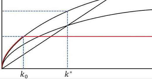
So given the model above we can now find out what different aspects do to economic growth given the model. If we are starting off in an initial steady state as shown below we can see that we hit a put where both sY and δK hit the put of equilibrium this is known as the steady state at this point the economic has hit it’s optimum growth limit this means that on a change in the variables  sF(Kt ,L) or δKt can either decrease or increase the long run level of economic growth.

Now as stated above we can see we are at a steady state level within the economy, and this is where the economy will stay unless there are changes to variables within the model. So, we we had a rise in sY to s’Y thus we add more new investment that is greater than the rate of deprecation we get a new steady state and thus a higher level of growth within the economy as shown below. This is currently the state in the United States. Below will be shown a photo of deprecation as well as that of the steady state.

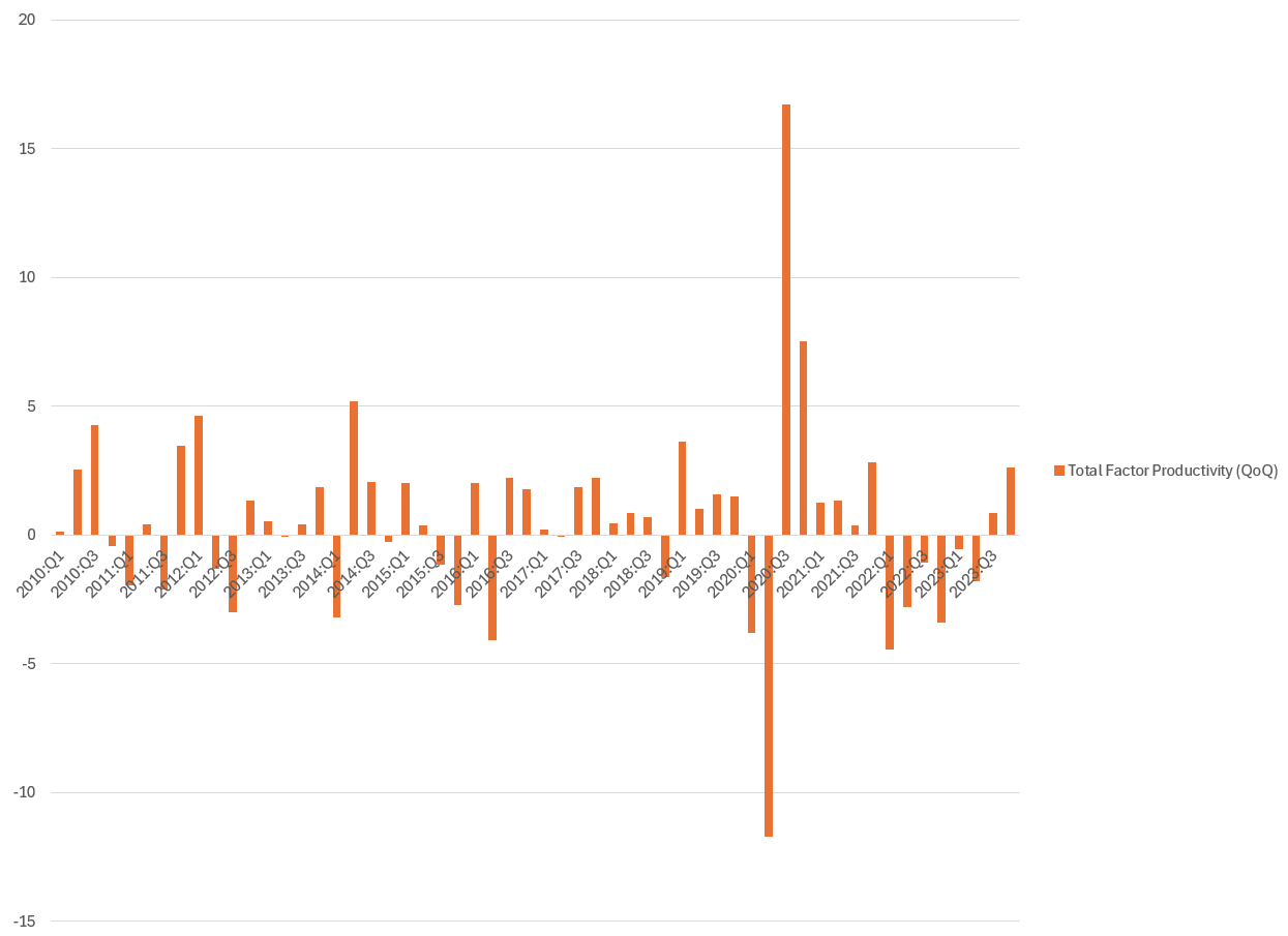
After the massive Total Factor Productivity (TFP) growth we witnessed in the US today, examining the Solow Residual and its contribution to overall growth for the United States becomes crucial, not just at the output level but also in increasing standards of living.

It's worth noting that Robert Solow had the expectation that as the fertility rate falls, we should start to see increases in technological progress. The decline in overall fertility rates, coupled with the increase in overall technological progress, should enhance the overall level of output and lead to increases in the efficiency of capital.

All of this amounts to higher levels of output, which should help lift the per capita income of Americans.

Now, the growth model is extremely important for understanding the increase in the overall standard of living. When we examine the Residual, which in simplistic terms represents growth generated that does not stem from increases in labor or capital, we observe a rise in US growth.

In analyzing this model, it's essential to recall that alpha equals 0.3 in the Cobb-Douglas production function. Despite this, we can discern an increase in the overall Residual, contributing to higher levels of GDP per capita. This, in turn, enhances the standard of living, although GDP per capita might not be the preferred measure of economic well-being.

Given the current rise in the Residual, expectations are for US growth and standards of living to continue improving. This serves as another bullish signal for the US economy and is expected to translate into higher levels of domestic consumption.

Now, let's shift our focus to GDP. The bears have been emphasizing the notion that GDI is falling. However, we need to delve into disproving this bearish statistic and examine the problem with GDI.

Net national savings as a percentage of GDP is negative for the US, but this metric is misleading. It subtracts depreciation from the numerator but not the denominator, thus shrinking the savings-to-income ratio. We can observe that the orange line falls much faster than the purple one. This is because depreciation has risen. Over the last 50-60 years, we have witnessed a shift in the capital stock. Technological advancements or factors that increase Total Factor Productivity (TFP) tend to depreciate faster than, for instance, structures. Because net national savings subtracts this from income but adds it to savings, this results in more downward momentum than would otherwise be the case.

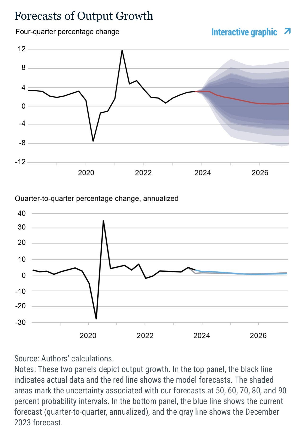
The NY Fed has revised Q1 growth up from 1.2% to 1.9%, indicating the continued strength of the US economy.

The Fed's Dynamic Stochastic General Equilibrium (DSGE) model forecasts GDP growth of 1.9% in the first quarter of 2024. This marks a revision up from 1.2% in December and was primarily driven by the increase in productivity growth and favorable financial conditions, which the model considers as contributors to forecast error (1.2%). This is pointing to an overall increase and positive outlook in the United States economy.

US GDP appears poised to sustain its strong momentum. Before the pandemic, the model had an R-squared of 0.79. However, due to the pandemic, the correlation has broken down, now standing at around 0.46. Nevertheless, with the expectation of normalization, factors such as US Total Factor Productivity (TFP) growth and the increase in investment relative to depreciation have moved the steady state higher. Considering these factors, US growth should continue to benefit throughout the remainder of the year.

Now let's shift our focus to the inflation picture in the United States. Demand remains robust, but we are observing a decline in the marginal propensity to consume. This trend has historically followed changes in overall demand-driven Personal Consumption Expenditure (PCE) inflation. As a result, we should start to see a gradual easing of the overall output gap and, consequently, inflation.

The easing of demand-driven inflation is expected to continue fading throughout the remainder of the year. Additionally, as supply continues to come online through near-shoring, this should help readjust the output gap. This adjustment will entail a rightward shift in the aggregate supply curve, allowing supply to meet demand. Eventually, the inelasticity in the supply curve kink will begin to resolve itself.

Now looking at the overall makeup of drivers of inflation Supply- and Demand-Driven Contributions to Annualized Monthly Headline PCE Inflation we are seeing overall easing of most areas of inflation both demand, ambiguous, but supply-side continues to be elevated. As mentioned above the overall increase in productivity and the nearshoring should help to stabilize this and readjust the output-gap. Below is shown the output-gap relative to supply inflation. The graph below that is the overall contributions aggregated.

Now a bit of an explanation of the output-gap. This is essentially a measure of supply and demand. When the output-gap is positive that means demand is higher than supply, and thus you have a positive output gap. This can happen for many reasons but the main driver was built up demand throughout the pandemic which is still working itself out. As excess savings comes down this should start to come off and thus reduce the output gap. However, that excess demand takes a while to work through the system. Thus lagging the overall aspects pointed out above. However, it is an important metric to analyze.

Coming into the 2H of 2024 I expect us to see more decreases in supply and given the output and productivity numbers I think this is a good bet, and thus any expectation of higher and stickier inflation should be faded.

Now, let's analyze the overall level of production in the United States, considering the two parts of the equation for the steady state. The Solow growth model equation can be represented as:

Kt+1​=sAKtα​+(1−δ)Kt

Alternatively, this can be expressed as the change in capital stock over time:

Kt+1​−Kt​=sAKtα​−δKt​

First, let's examine the right-hand side of the equation. δKt represents depreciation, while sAKtα ​represents investment in new capital. When α=1/2, the term Kαt​ essentially signifies the square root of capital Kt​. Graphically, this translates to a curve that initially slopes upward but flattens out over time.​

Increasing A in the equation would shift the steady state, resulting in Kt+1​>Kt​, indicating that capital investment surpasses depreciation. Consequently, this leads to an increase in output Y′, investment I′, and consumption C′ compared to prior levels as the economy transitions to a new steady state. Eventually, the capital stock stabilizes when Kt+1​=Kt​, signifying the attainment of the steady state.

The current state of the US economy reflects a permanent increase in A and other factors influencing total factor productivity (TFP), leading to higher levels of output, investment, and possibly consumption. This shift results in the economy operating at a higher level represented by K∗. While the linear line represents δKt​, the increase in A causes a shift in sAKtα​, indicating that Kt+1​>Kt​. This trend is evident in the chart, where capital stock investment is growing more rapidly than the rate of depreciation, consequently boosting overall productivity in the United States.

The driving force behind this phenomenon appears to be the rise in total factor productivity A or TFP, which is altering the steady state and leading to a situation where Kt+1​>Kt​. When the purple line is positive capital stock investment > deprecation or Kt+1>Kt.

In economics, there is a concept I've discussed extensively throughout this post known as Total Factor Productivity (TFP). It's often regarded as economic magic, albeit subject to debate within economic circles. I adhere to the perspective that TFP measures technological progress. Mathematically, it is explained through the production function:

Y=AL^aK^b

Where a+b=1 and (a,b) lies between (0,1). Changes in A signify shifts in the relationship between measured aggregate inputs and outputs, with proponents believing that changes in the variables are induced by technological advancements. To measure this, the stock of inputs is considered over the long run, along with deviations in capacity utilization. To derive the geometric version of TFP, we divide both sides of the production function by L^aK^b to obtain:

TFP=Y/L^aK^b​=A

In simpler terms, TFP represents the productivity of all inputs or factors of production in relation to their aggregate effect on output. It's typically associated with changes in technology, leading to more efficient methods of output. TFP effectively measures the long-term growth of an economy.

In the last quarter, we witnessed a significant boost in TFP. This surge appears to stem from various factors, with a significant driver being investment and technological advancements that enhance overall output levels or, in other words, output efficiency. This surge has played a substantial role in driving US economic growth over the past few quarters, and I anticipate this trend will persist, particularly given the focus on supply-side policies.

Now sticking with the productivity boom lets look at the effect that this has had on corporate profits. Productivity=Profits we have seen a huge increase in corporate profits without inventory adjustments coming increasing by almost 400bps. Despite all the worries surrounding higher rates, inflation, and other aspect we have not seen detrimental effect on business expansion in the United States.

If you want to know where profits will go one should simply focus on the overall changes in productivity. As productivity has expanding we have seen a rapid rise in profits. This is why despite all the negativity surrounding US equity growth and the possibility of slowing business expansion I think these worries are overblown. As productivity continues its growth as will profits.

In terms of aspects that remain bullish I think anything tied to the real economy should continue to perform well, especially on the back of the productivity boom that we are seeing in the United States.

Next looking at corporate profits after tax and GDP growth is also a good indication of the overall health of the economy. The health of overall domestic corporations continues to look healthy, and this is driving and will continue to drive equity market growth. When the economy is ripping consumers will continue consumption as well as business activity will continue to be robust. This means more investment and CAPEX spending. We will also tend to see a tighter labor market as growth continues to pick up and companies want to make sure they can meet the overall demand from consumers. We should as well see higher levels of capacity utilization.

The chart below shows that there is a close relationship between profit growth and GDP within the US. Given that corporate profits are rising this should continue to act as a positive impact on the US economy as well as US GDP into the remainder of the year. Thus do not try short domestic activity.

It is important to note that this relationship is not perfect. There are things within the graph that can lead to overall divergence. However, it continues to show positivity and positive outlook on the US economy.

The final aspect that I want to touch on is the equity market and corporate earnings. When earnings pick it seems though equity prices continue to rise. During the 1990s earnings peaked as a percentage of GDP in 1997 while stocks continued to rise until 2000 (CME Group, 2015). During the following 10 years earnings peaked relative to GDP in 2006, but equities did not reach their highest level until 2007 (CME Group, 2015). This also happened in 2011-14 where earnings peaked and then began falling, and we saw continue upward growth in equity market (CME Group, 2015).

Now the measure to watch is that of the VIX as post-peak earnings often coincided with increased levels of rising equity volatility (CME Group, 2015). Now that the overall level of equity vol. remains suppressed and we are seeing increasing corporate earnings I would not worry to much currently about a peak in corporate profits as a percent of GDP. This is a decent indicate to track for further increases in growth.

In conclusion the United States economy continues to be a powerhouse, and continues to be the leader around the world. While many economies are slowing the United States economic activity continues to remain robust. This gives me faith that the United States should continue to see very high levels of economic activity, and moderating to declining levels of inflation. Those who are betting against the United States are standing in front of a runaway train. The overall outlook continues to give me optimism about the United States in both the short and long-run.