Everything Macroeconomics

Introduction
This post will examine the current macroeconomic backdrop of the United States, highlighting key dynamics shaping the economy and markets. We will explore trends in GDP, growth, and output, while also analyzing the interplay between the current and capital accounts. Finally, we will connect these fundamentals to what is unfolding across financial markets today.
GDP
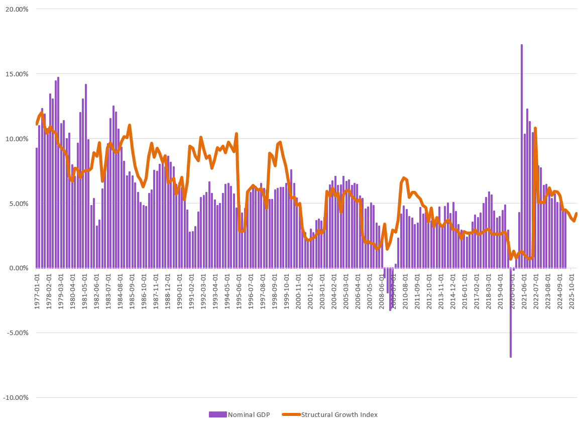
U.S. GDP grew 0.78% month-over-month, reinforcing the view that recessionary pressures are not yet evident. Importantly, we have been developing an income-based approach to GDP measurement, which offers a distinct advantage: while the traditional expenditure approach is only available on a quarterly basis, income-side data is published monthly. This higher-frequency lens provides earlier insights into underlying economic momentum and allows us to assess turning points in activity ahead of the standard GDP release.

1/ PK growth law:
g = s_p * (ROA − r_D) / ν
s_p=1−payout, ν≈PPE/Revenue.
Growth comes from reinvested profits earning above debt cost, scaled by capital intensity.
The PK growth law says corporate growth comes from retained profits.
If companies keep profits (instead of paying them out), they reinvest.
If the return on those assets (ROA) is greater than the cost of debt (r_D), reinvestment is productive.
The capital-output ratio (ν) shows how much output you get per unit of capital — higher efficiency means more growth.
This gives you a measure of how much growth the corporate sector can generate on its own, without needing outside borrowing or policy support.
2/ GDP link:
Treat g as the internally financed piece of ΔY/Y. If g < GDP, consumption/fiscal/trade are doing more work; if g ≈ GDP, corporate reinvestment is the driver.
The PK growth law isolates the investment piece — the part of GDP growth that can be explained by corporate reinvestment of retained earnings.
If PK ( g < GDP):
GDP growth must be coming from consumption, government, or trade more than corporate reinvestment.If PK ( g ≈ GDP):
It means corporate reinvestment is the main growth engine.If PK ( g > GDP):
It suggests corporations are expanding faster than overall demand, which can lead to overcapacity or adjustment later.
Currently g>GDP which points to corporations expanding faster than overall demand, which could lead to overcapacity and thus we could face a negative output gap at some put in the future. This is good on the inflation front, as we would see disinflation.
This is also positive on the investment front as it will lead to higher potential output, excess capacity, disinflationary pressures, and if demand increases or stays stable higher future growth granted demand shifts to the right with incremental increases in output.
The headwind is if demand shifts to the left you get lower growth until that demand catches back up.
The idea to try to model this came from a post I saw on twitter, but cannot remember the person who first brought this idea front and center, but credit to them anyways for helping lay the ground work to attempt to model this.
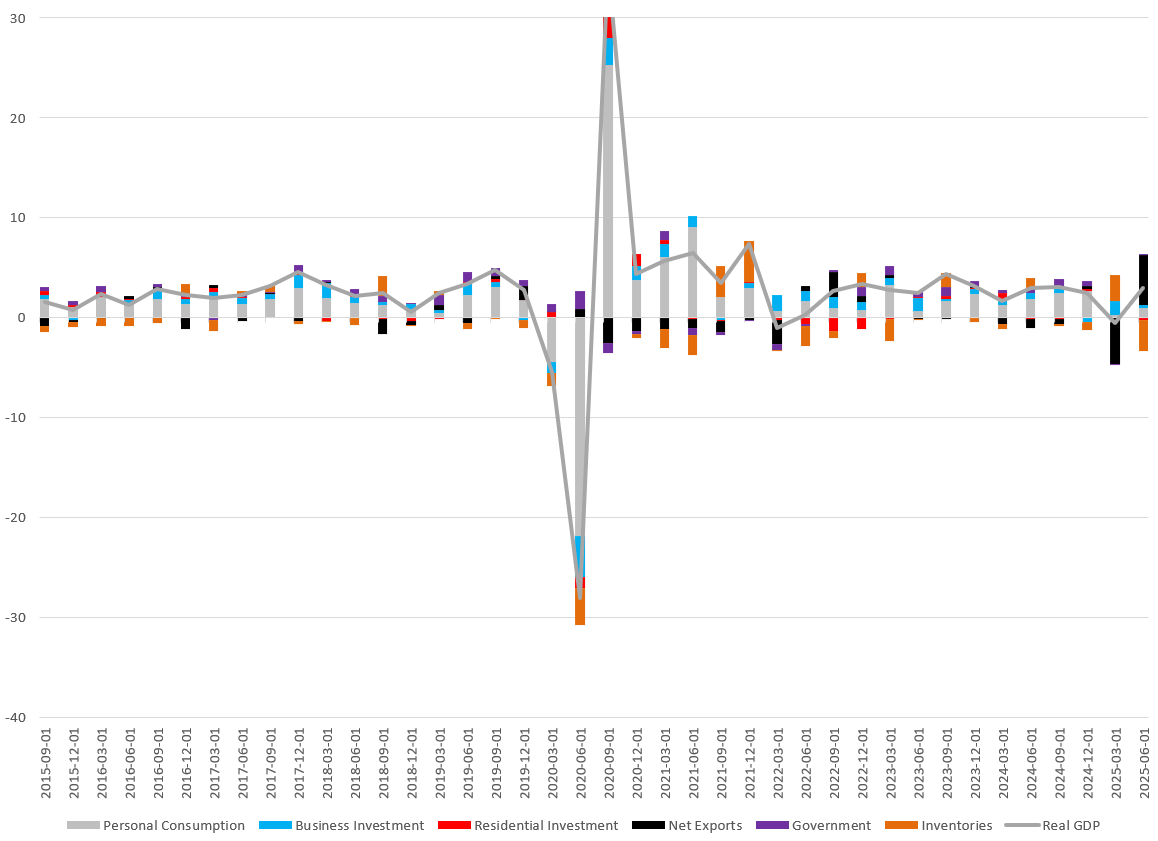
Current drivers of real GDP. In Q1, we saw significant stockpiling of inventories alongside a surge in imports. Over time, this tends to average out—purchasing a good from overseas (an import, which subtracts from GDP) is eventually offset when that same good is consumed (which adds to GDP). In theory, this should result in no net impact on GDP, since the good was not produced domestically. However, in Q1, the negative effect appeared without the corresponding positive offset.
A rush to beat tariffs boosted imports in the first quarter, leading to a record goods trade deficit that weighed on the economy. That trend reversed in the following quarter, as imports declined sharply, reducing the trade deficit and adding 4.99 percentage points to GDP. This more than offset the 3.17 percentage point drag from inventories.
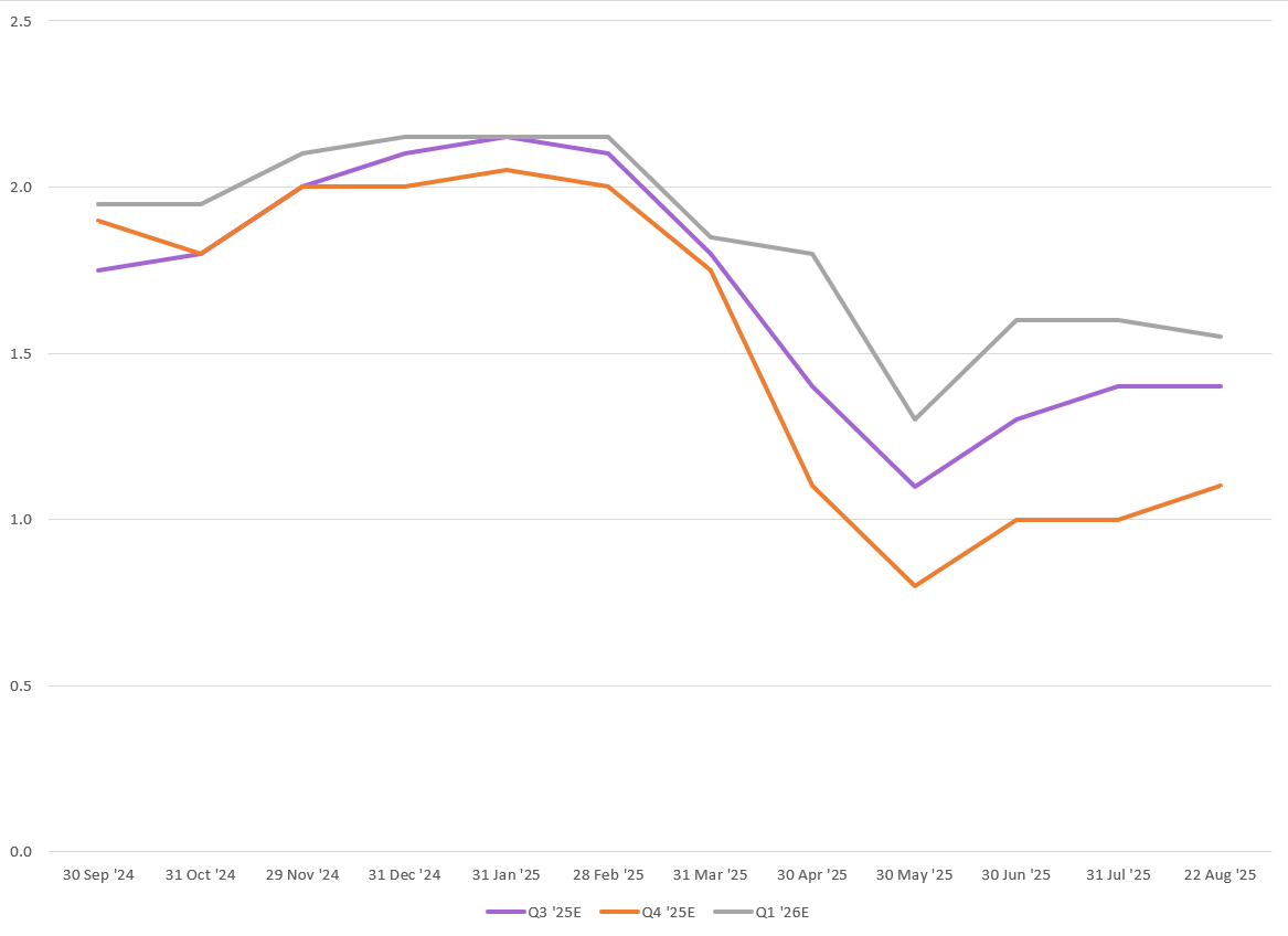
Forecasts for real GDP growth - quarterly is being revised up currently expectations of around slightly under 1.5%.
Long-Run Driver of Growth
We will examine the overall framework of the exogenous growth model and its implications for changes in the steady state of the United States economy. It is important to first understand the mathematical foundations of the model, as they provide insight into how growth dynamics evolve over time.
Let us define the key terms:
Yt: output at time t
Kt: capital stock at time t
Lt: labor input at time t
It: investment at time t
A: total factor productivity (TFP)
L: labor force
K0: initial stock of capital
δ: capital depreciation rate
s: savings (or investment) rate
n: population growth rate
g: labor productivity growth rate
The production function is given by:
Yt = F(Kt ,Lt)
Capital accumulation in period t + 1 is defined as:
Kt+1 = Kt +It −δKt
Rearranging, we obtain:
∆Kt+1 = It −δKt where ∆Kt+1 ≡ Kt+1 −Kt
This illustrates that the accumulation of capital in each period depends on the balance between new investment and depreciation of existing capital. Since investment is a fraction of output (It = sYt), consumption is given by:
Ct = (1−s)Yt
Substituting, we arrive at the capital accumulation equation:
∆Kt+1 = sF(Kt ,L)−δKt
This formulation gives us the foundation for the exogenous growth model and allows us to derive the steady state.
At the steady state, investment (sY) exactly offsets depreciation (δK), leaving no further net capital accumulation. The economy, therefore, converges to an equilibrium where output, capital, and consumption grow at constant long-run rates.
However, changes in parameters such as the savings rate (s) or depreciation rate (δ) can shift the steady state. For example, if the savings rate rises from sY to s′Y, investment exceeds depreciation, leading to a new steady state with a higher long-run level of capital and output. This mechanism highlights why the savings and investment rate is one of the most critical determinants of long-run growth.
In the context of the United States, current dynamics suggest that changes in savings and investment behavior are moving the economy toward a higher steady state, reinforcing the importance of capital deepening as a driver of sustained growth.
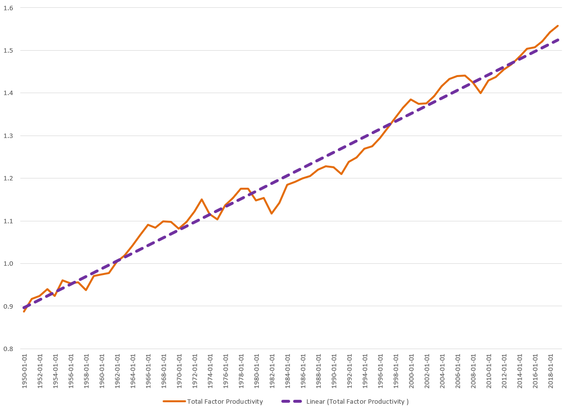
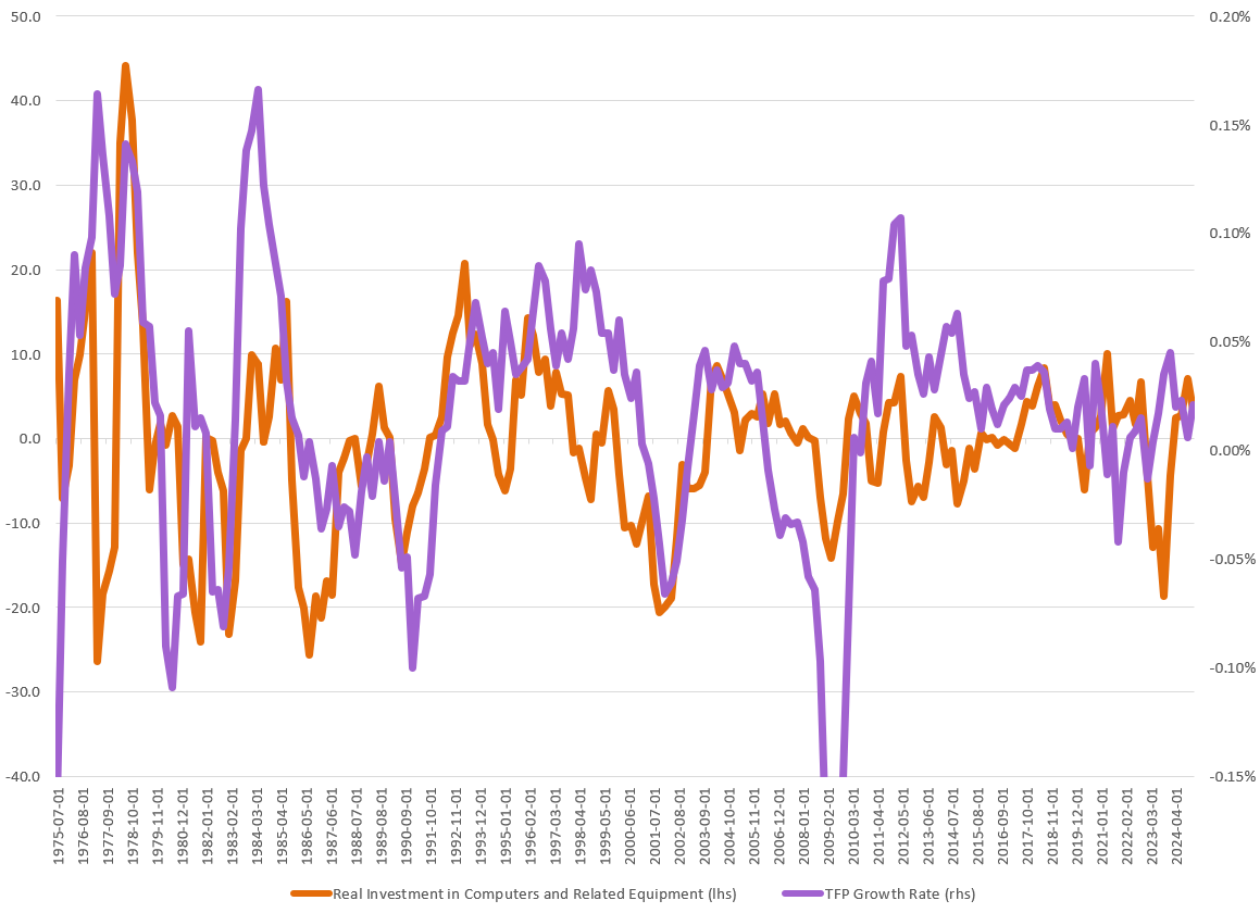
Investment in computers other equipment related to computers saw quiet the drop rising around 10% YoY. We can see from the last 20 years we are currently above trend of the last 2 decades of investment. Computer investment will continue to be a large driver especially given the backdrop of the AI boom. Computers can make labor more productive through automation, data processing, and that is a capital-labor complementarity, not just substitution. Adding computers and other equipment increases measured K. When output rises more than expected from K and L increases, the excess goes into A (TFP). IT is often credited with a TFP surge: it has broad, complementary effects that go beyond simple capital accumulation.
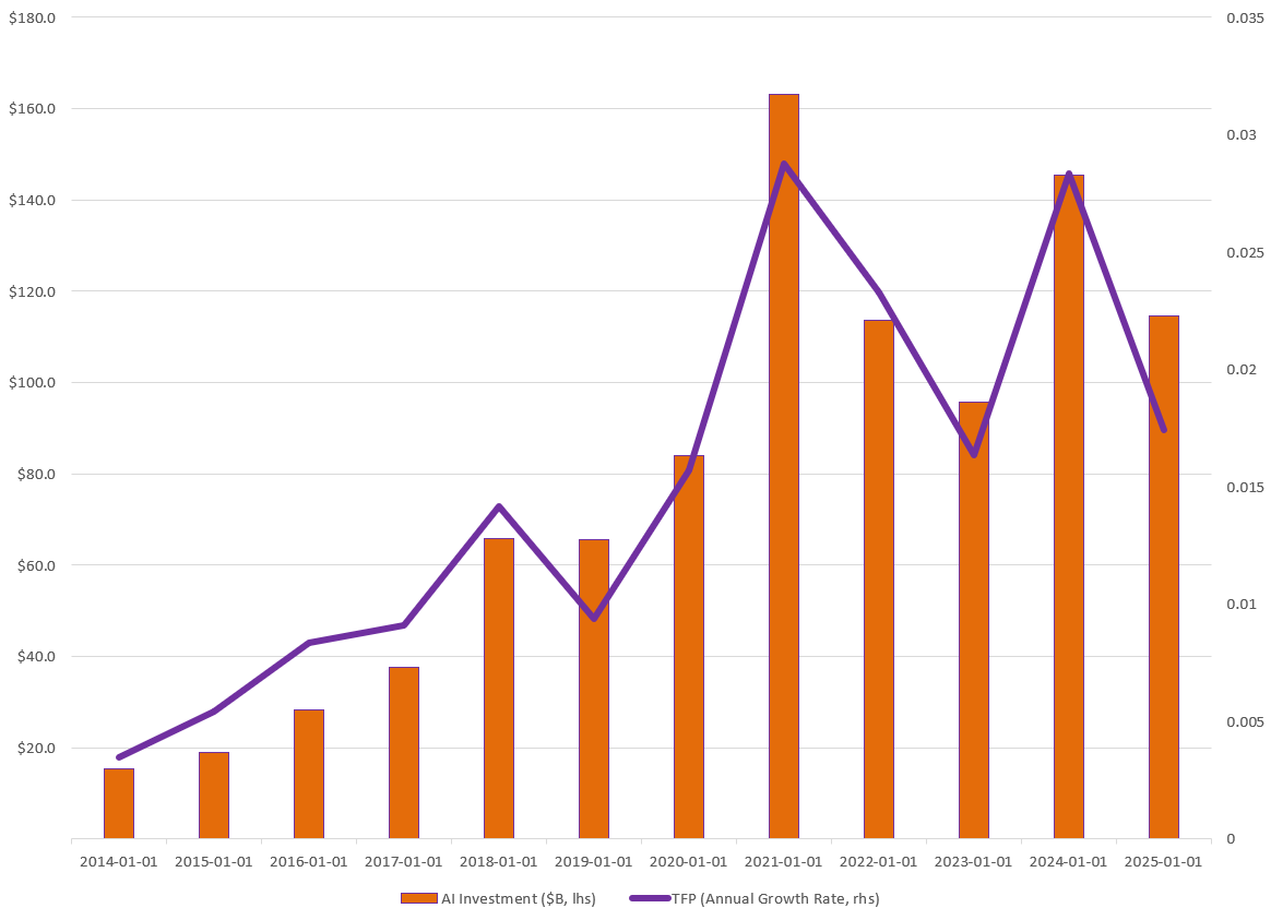
Increased AI investment can boost total factor productivity (TFP) by enabling firms to produce more output with the same amount of labor and capital. AI enhances efficiency through automation of routine tasks, improved data-driven decision-making, and optimization of production processes. It also generates spillover effects, as firms adopting AI often stimulate innovation and productivity gains across supply chains and industries. Over time, these benefits show up not as larger inputs, but as higher residual productivity growth the part of output expansion not explained by capital and labor alone.
Capital Flows
When people talk about what drives long-term interest rates, the focus is usually on inflation expectations, Federal Reserve policy, and the term premium investors demand for holding longer bonds. But another piece of the story is international demand: how much foreign investors are buying U.S. Treasuries relative to the size of the economy.
To test this, I ran a regression of the 10-year Treasury yield on:
Long-term (10y) inflation expectations
Short-term vs. long-term inflation spread
The Fed funds rate
The risk premium
Expected real GDP growth
The lagged budget deficit (% of GDP)
Lagged foreign capital inflows (% of GDP)
This setup follows the intuition that long-term yields reflect both fundamentals and the balance of supply/demand in bond markets.
The math for the model follows:
Scale and lag:
flows_pct_gdp_t-1 = capital_flows_t-1 / gdp_t-2
deficit_pct_gdp_t-1 = (budget_deficit / gdp)_t-1
Inflation Reparam:
Δπ_t = π^e_1y,t - π^e_10y,t
Regression Equation:
y10_t = α+ β1*π^e_10y,t+ β2*Δπ_t+ β3*ff_t+ β4*tp_t+ β5*y^e_t+ β6*deficit_t-1+ β7*flows*_t-1+ ε_t
Where:
y10_t= 10-year Treasury yieldπ^e_10y,t= 10-year inflation expectationsπ^e_1y,t= 1-year inflation expectationsff_t= federal funds ratetp_t= risk premiumy^e_t= expected real GDP growthdeficit_t-1= lagged budget deficit as % of GDPflows*_t-1= lagged foreign inflows as % of GDP
Estimation:
β̂ = (X'X)^-1 * X'y
ŷ10_t = X_t * β̂
ε_t = y10_t - ŷ10_t
Impact Series:
Impact_t = β̂7 * flows*_t-1
Marginal Effect:
Δy10 ≈ β̂7 * Δ(flows*)
Results:
If Δ(flows*) = +1% of GDP
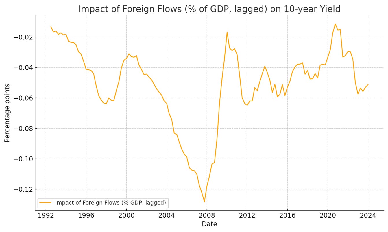
and β̂7 = -0.073
then Δy10 ≈ -0.073 (~ -7 bps)
The end results of this are that capital inflows tend to lower yields modestly. If foreign inflows rise by 1% of GDP, the 10-year yield is about 7bps lower. The larger the foreign purchases of U.S. bonds you can get rally in yields on the long-end. Obviously this will vary with time, and the ways one models the data.
The Fed inspired my own modeling of this from a paper called, “International Capital Flows and U.S. Interest Rates” by Francis Warnock and Cacdac Warnock. The impact they found was much larger with a 1% increase in flows leading to a -23bps move in the 10y.
Nevertheless what we can conclude is that foreign demand can help keep interest rates low, borrowing costs low, and help increase demand in assets that tend to be amortized over a long period of time.
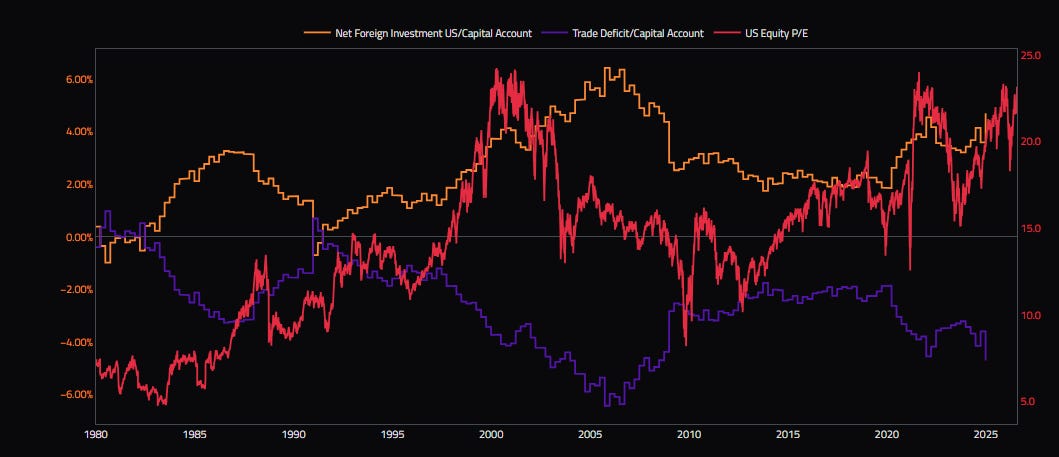
This chart shows the demand for long-term securities, which broadly mirrors the current account (note: there is a typo on the graph). When discussing the current account deficit, I would argue that it stems from the demand—or bid—for U.S. securities, rather than the other way around. In other words, it is the demand for our securities that drives the deficit. Any shift away from this demand, or an increase in uncertainty, could have significant effects on the bid for U.S. assets. A decline in demand for U.S. debt would not only disrupt capital flows but also place upward pressure on yields.
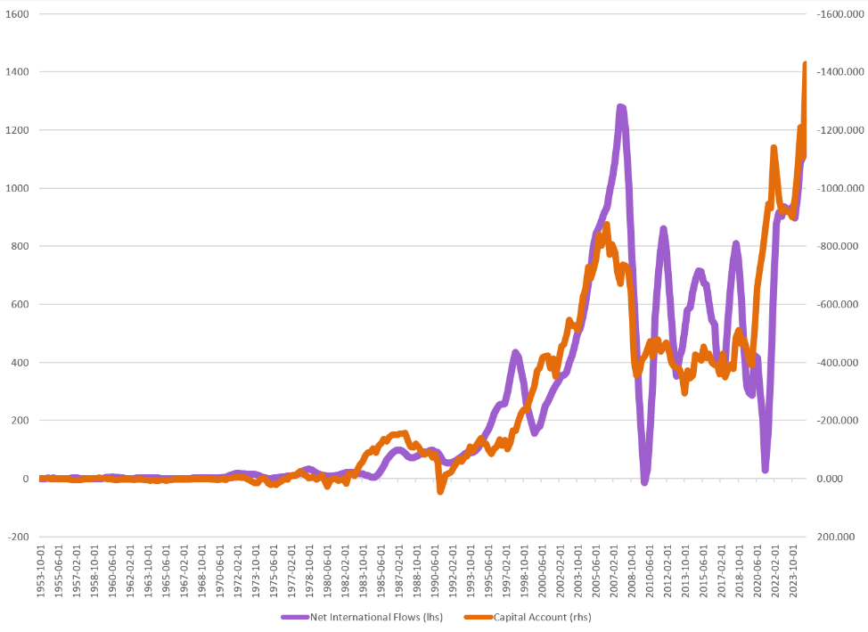
The trade deficit reflects the inflow of foreign capital into the United States, which has supported higher asset values. A narrowing of the trade deficit would imply a reduced flow of foreign capital, placing downward pressure on capital markets. Unless offset by an increase in domestic savings, such a decline could put valuations at risk.
Quadrants
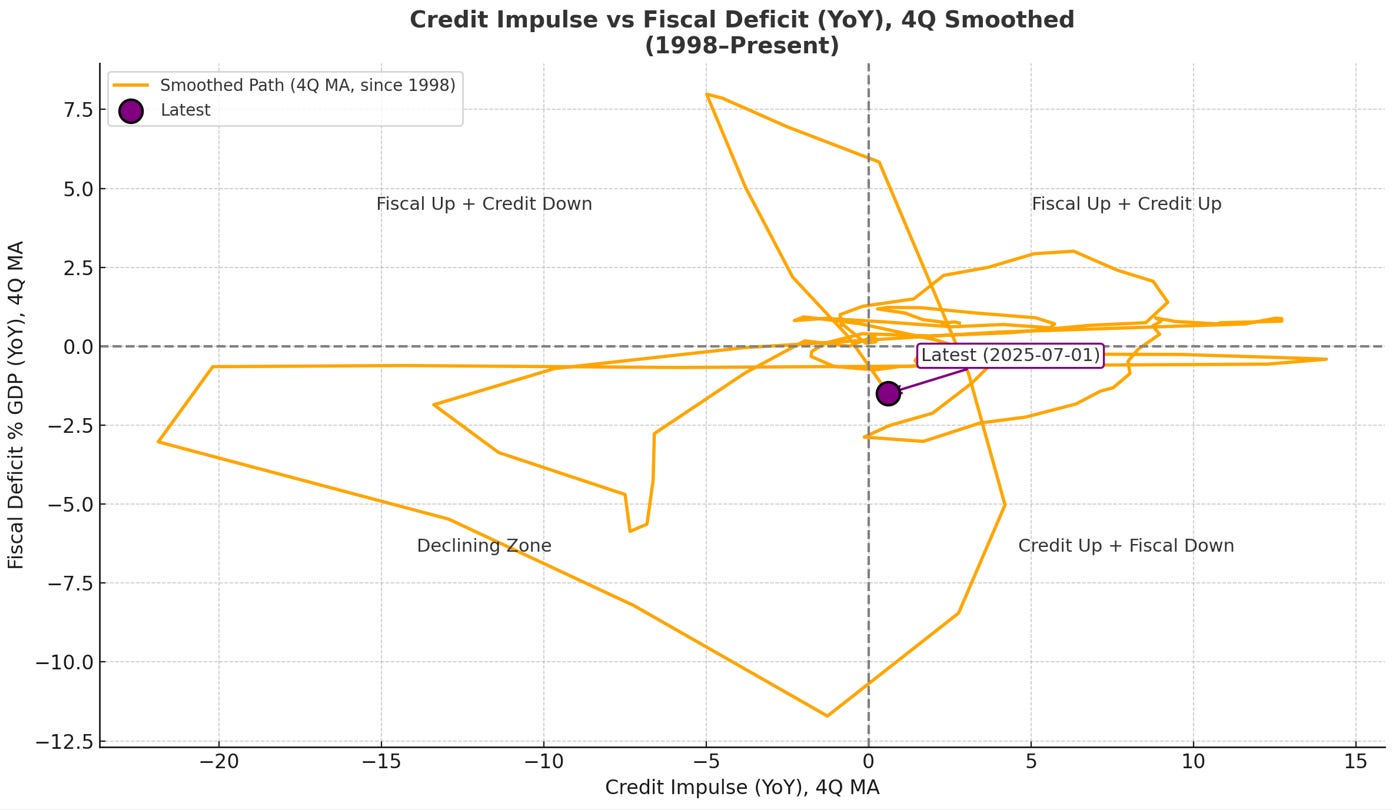
Below was inspired by a conversation with Doug (@mmtmacrotrader) on X. Since 1998, we can track the progress of credit and fiscal dynamics. For a while, we were in the upper-right quadrant, before shifting into a period of declining fiscal and declining credit. From there, we moved back into credit up + fiscal down, then into fiscal up + credit down, and now we have returned to credit up + fiscal down.
One of the risks going forward, as Doug highlighted in our conversation yesterday, is that fiscal is essentially flat while credit is accelerating—conditions that can lead to a bubble. Fiscal policy generally has a stronger impact on the economy than credit, but when credit impulse increasingly drives activity, it raises the risk of entering the bubble zone.
Is this the end of the world? No. But, as Doug also pointed out, the key will be whether by 2026 we can shift back into the upper-right quadrant.
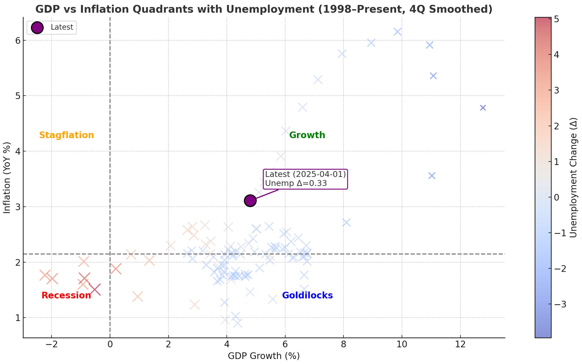
The chart above places the U.S. economy in a GDP–inflation–unemployment quadrant framework since 1998. GDP growth is shown on the x-axis, inflation on the y-axis, and changes in unemployment are captured in the color and size of the markers. The purple dot highlights the most recent observation (Q2 2025).
GDP Growth: Still firmly positive, running above trend.
Inflation: Moderating from its post-pandemic highs, but not back to pre-2020 lows.
Unemployment: Rising only slightly (Δ ~0.3pp), which suggests a modest cooling but far from a sharp deterioration in the labor market.
This places the economy in the Growth quadrant rather than in stagflation or recession. Inflation is above its long-term median but not accelerating, while output growth remains positive.
Stagflation, by definition, requires weak or contracting growth alongside persistent inflationary pressure. While headline inflation remains above the Fed’s 2% target, real activity has not slipped into negative territory. Instead, growth has been resilient, supported by consumer spending, fiscal policy, and private investment.
There are, however, two risk channels to monitor:
Labor Market Slack – If unemployment begins to rise meaningfully while growth slows, the economy could shift leftward on the chart, raising stagflation fears.
Supply-Driven Price Pressures – Commodity spikes, supply chain disruptions, or policy-driven cost shocks could keep inflation elevated even as output decelerates.
Right now, the data suggest we are in late-cycle growth, not stagflation. The “stagflation scare” narrative is premature—GDP momentum remains intact and the unemployment drift is small. Still, vigilance is warranted. If growth decelerates into 2026 without a parallel easing in inflation, the quadrant could shift toward stagflation risk.
For now, the more relevant concern is whether the Fed will allow inflation to remain sticky while credit continues to expand. That combination could eventually tip the economy toward instability, but stagflation is not the base case today.
Conclusion
Looking ahead, the U.S. economy appears set to remain broadly resilient, even as growth slows into 2026. While inflationary pressures have moderated and remain on watch, the balance of risks does not point toward a stagflationary environment. Instead, the more likely trajectory is a gradual deceleration in activity as higher interest rates and tighter financial conditions filter through the economy, while labor markets and household balance sheets provide an offsetting source of strength.
Importantly, the underlying macro backdrop remains stable. The U.S. continues to benefit from strong institutional frameworks, deep capital markets, and an ongoing bid for dollar assets, all of which mitigate the likelihood of a sharp dislocation. Fiscal dynamics and credit conditions will play a role in shaping the pace of slowdown, but neither appears to present systemic risk at this stage.
Overall, while the pace of expansion is expected to ease in the coming years, the probability of a disruptive stagflationary scenario remains low. The outlook is best characterized as one of slowing but resilient growth, where macro risks are present but contained. In this environment, the U.S. continues to stand out as relatively stable compared to many other advanced economies, with negligible near-term macroeconomic vulnerabilities.